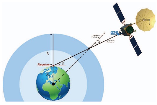
Figure 1. Geometry of Satellite-Receiver.

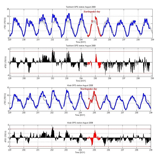
Figure 2. TEC anomaly for the Tashkent EQ occured on 22-Aug-2008.

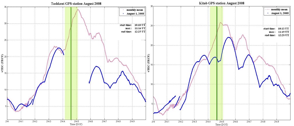
Figure 3. Variation of TEC amplitude for Tashkent (left panel) and Kitab (right panel) GPS stations during the Solar Eclipse on 01-Aug-2008.

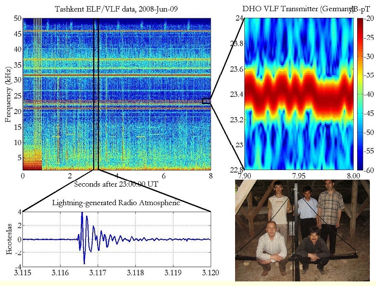
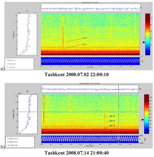
Figure 4. Data taken with VLF antenna in Tashkent. The top left plot shows a spectrogram, in which the frequency content is divided for individual time bins, and the strength is indicated by the color scale. The bottom plot shows a time-series zoom-in of a radio atmospherics, i.e., short impulsive radiation from a lightning stroke which may be at global distances. The right plot shows a VLF transmitter signal, in this case originating from Germany, with the MSK communication signal evident by the up and down frequency changes. Since both the radio, atmospherics and the VLF transmitter signal rely on the D-region for propagation, the received signals are both extremely sensitive to the various ionospheric disturbances described herein.

Figure 5. Examples of dynamic spectrograms of tweeks observed during the nighttime at Tashkent VLF station on July 2008.

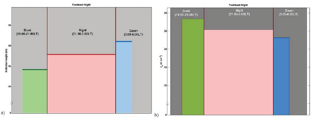
Figure 6. a and b figures show the ionospheric reflection height (in km) and electron density at these height (in el/cm3) at Tashkent VLF site, correspondingly.

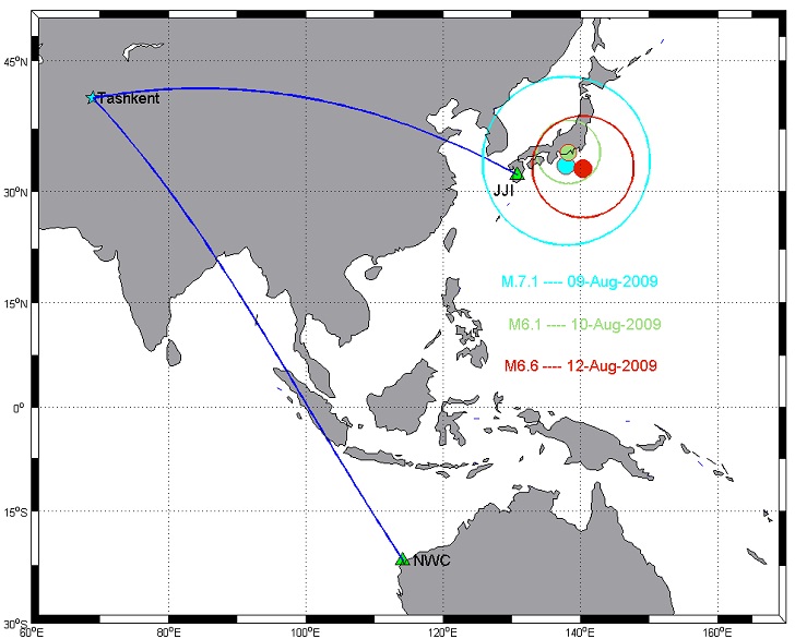
Figure 7. Map for Tashkent VLF station and Japan earthquakes epicenters.

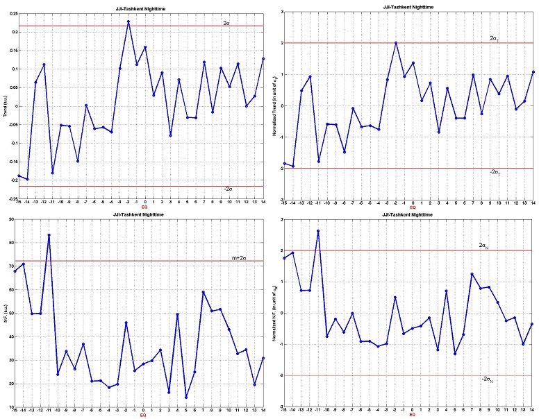
Figure 8. The nighttime average amplitude(or trend) and nighttime fluctuation variation for Japan EQ on 09-Aug-2009. Top panel indicates trend (left) and normalized trend (right). Bottom panel indicates N.F.(left) and normalized N.F. (right).

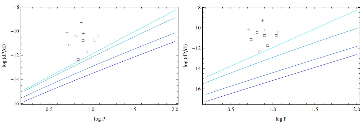
Figure 9. The picture of deathlines for rotating and oscillating magnetars